Opencv 图像处理
Published: 2020-03-17
Finding Lane Lines #
#importing some useful packages
import matplotlib.pyplot as plt
import matplotlib.image as mpimg
import numpy as np
import cv2
%matplotlib inline
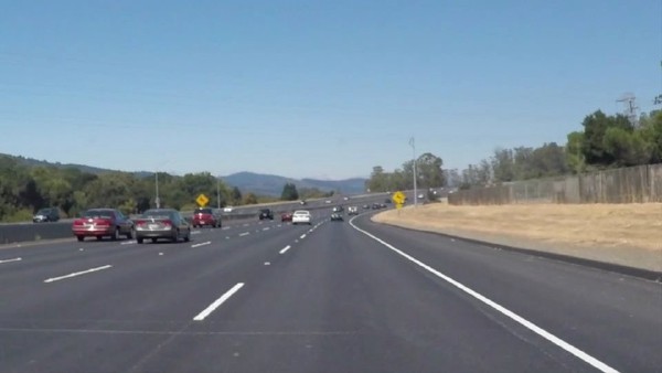
在原图像中找到车道线,需要进行5步操作:
#reading in an image
image = mpimg.imread('test_images/solidWhiteRight.jpg')

# if you wanted to show a single color channel image called 'gray',
# for example, call as plt.imshow(gray, cmap='gray')
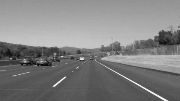
plt.imshow(image)- converted the images to grayscale.
cv2.cvtColor(img, cv2.COLOR_RGB2GRAY)
# Or use BGR2GRAY if you read an image with cv2.imread()- In order to eliminate the efffect of random noise, Gaussian blur method is applied to the image. The image is a little blurry after the operation, but it's benificial for the next step.
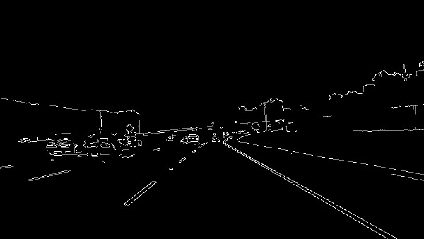
cv2.GaussianBlur(img, (kernel_size, kernel_size), 0)- Then, the canny algorithm is used for edge detection. Pixels with large gradients are likely to be lane lines as the color changes rapidly.
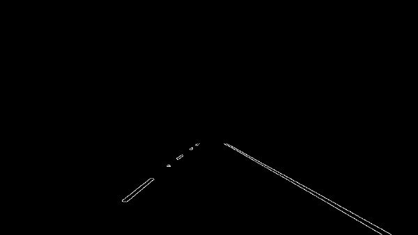
cv2.Canny(img, low_threshold, high_threshold)- Crop the Image. Lane lines are always right in front of the car, so only a small portion of the image needs to be processed.
#filling pixels inside the polygon defined by "vertices" with the fill color
cv2.fillPoly(mask, vertices, ignore_mask_color)
#returning the image only where mask pixels are nonzero
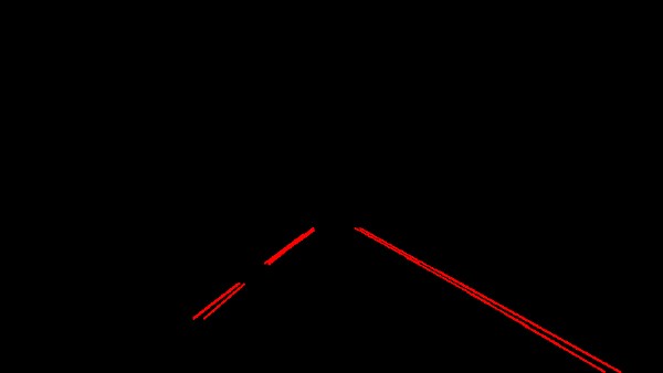
masked_image = cv2.bitwise_and(img, mask)- Hough transformation is really useful for line detection.
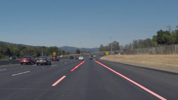
lines = cv2.HoughLinesP(img, rho, theta, threshold, np.array([]), minLineLength=min_line_len, maxLineGap=max_line_gap)when the detected lines are overlayed on the original image, we can see that the lane lines are detected sucessfully.
cv2.addWeighted(initial_img, α, img, β, γ)Advanced Lane Finding #
高级车道线检测需要在俯视图上进行,分为如下步骤:
Use color transforms and gradients to create a thresholded binary image.
I used a combination of color and gradient thresholds to generate a binary image.
R and G channels are used as they are helpful to find yellow lane lines, which is quite common in the real world. When image is converted to HLS channel, white and yellow lane lines are quite distinctie, and the influence of shadows can be significantly reduced.
Sobel gradient and gradient direction thresholds are also used, since the gradients varies most along x axis, and the lane lines are often vertical to the car.
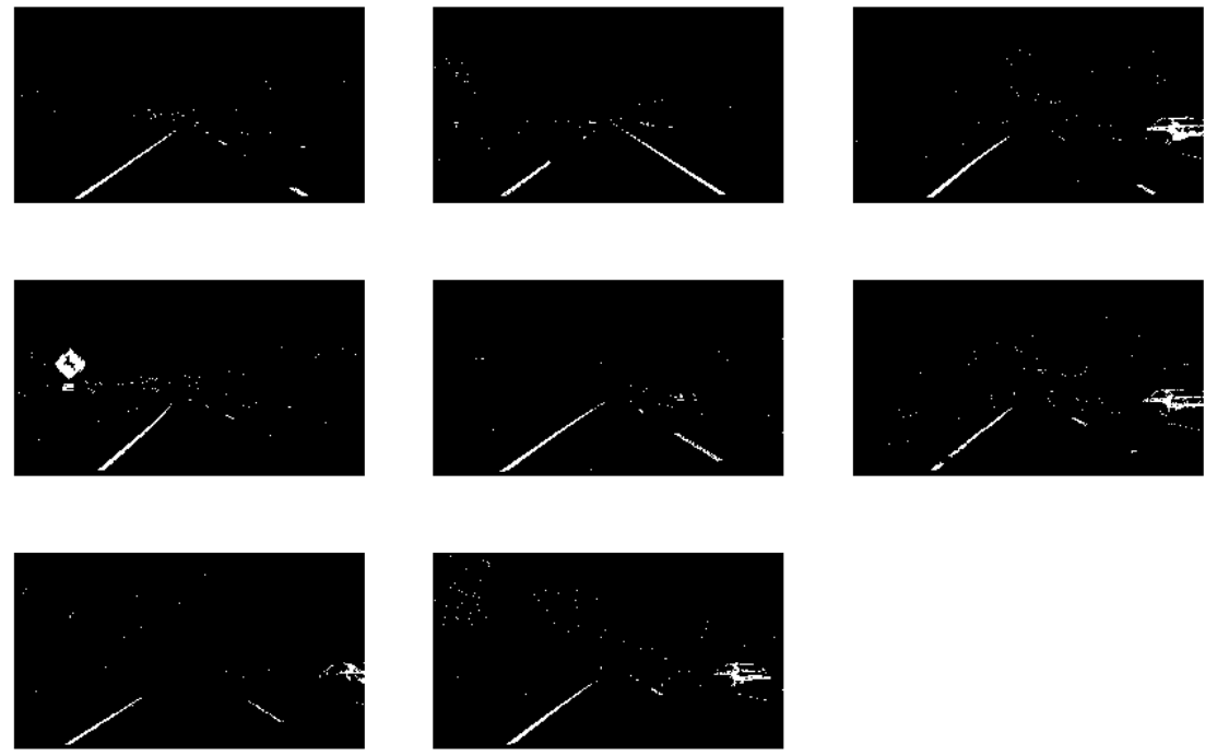
Here are some examples of test images when converted to binary image. The lane lines are preserved while most useless information is filtered out.
- Performed a perspective transform.
cv2.getPerspectiveTransform() function takes as inputs source (src) and destination (dst) points and is used to calculate perspective transform matrix.
Note that source points are chosen along the straight lane line to form a rectangle.
cv2.warpPerspective() function is used to rectify binary image.
I chose the hardcode the source and destination points as follows:
| Source | Destination |
|---|---|
| 570, 470 | 420, 1 |
| 722, 470 | 920, 1 |
| 1110, 720 | 920, 720 |
| 220, 720 | 420, 720 |
I verified that my perspective transform was working as expected by drawing the src and dst points onto a test image and its warped counterpart to verify that the lines appear parallel in the warped image.
- Identified lane-line pixels and fit their positions with a polynomial.
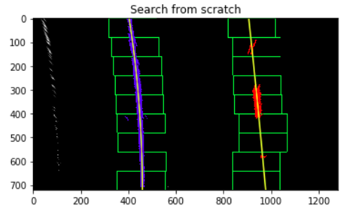
I first take a histogram along all the columns of the images, and the two highest peaks in the histogram are treated as starting point of the lane lines.
Then I used sliding windows to find all the possbile pixels in lane lines, and fit my lane lines with a 2nd order polynomial kinda like this:
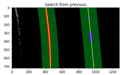
The position of lane lines shall not change much within seconds, so the polynomial derived from the previous image can be used as a starting point for the following image. Searching the lane lines along the previous polynomial can be much more efficient.
- Calculat the radius of curvature of the lane and the position of the vehicle with respect to center.
Firstly, we need to convert our calculation result from pixel world to real world.
Then, we can derive the real distance and curvature of the lane lines with a pre-defined formular.
I did this in the function curve_offset().
- Plotted back down onto the road such that the lane area is identified clearly.
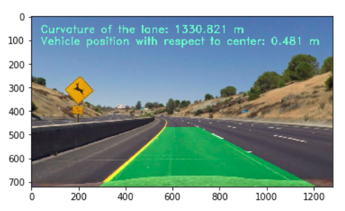
draw_lane() function is used to plot lane area back down onto the road, while draw_text() function is used to visualize numerical estimation of lane curvature and vehicle position.
Here is an example of my result on a test image:
Vehicle Detection and Tracking #
- Extract binned color, histograms of color, and Histogram of Oriented Gradients (HOG) features on a labeled training set of images.
- Normalize features and randomize a selection for training and testing.
- Train a Linear SVM classifier
- Implement a sliding-window technique and a HOG Sub-sampling technique. Then use the trained classifier to search for vehicles in images.
- Run the pipeline on a video stream (start with the test_video.mp4 and later implement on full project_video.mp4) and create a heat map of recurring detections frame by frame to reject outliers and follow detected vehicles.
- Estimate a bounding box for vehicles detected.
Data Visualization
In order to distinguish vehicles from non-vehicles, we need to collect as many data sets as possible. Udacity has provided us 8792 images of vehicles and 8968 images of non-vehicles. Here are some examples:
Feature Extraction
Since vehicles are significantly different with non-vehicles both in their shapes and colors, several kinds of features including binned color, histograms of color, and HOG are extracted from the datasets.
Binned Color Features
I used cv2.resize() function to resize the image from 6464 to 3232 to reduce the number of features. While others may resize the image to 16*16, I think it looks so blurry that even human can hardly recognize the vehicle. Here is an example of binned color features:
Histogram of Color Features
Histogram of color is also a good way to represent the property of an image and can be easily implemented with the function np.histogram. Here is an example:
Histogram of Oriented Gradients (HOG) Features
I grabbed the first images from each of the two classes and displayed them to get a feel for what the skimage.hog() output looks like. Here is an example using the YCrCb color space and HOG parameters of orientations=9, pixels_per_cell=(8, 8) and cells_per_block=(2, 2):
Train SVM Classifier
Combine and Normalize Features
I decided to extract all the features mentioned above and used np.concatenate() to combine them to a feature vector. As the magnitude of these features vary from each other, we should normalize the features and randomize a selection for training and testing.
Train and Test the Classifier
I trained a linear SVM using the training dataset and achieve an accuracy of 99.94% with the testing dataset. Although other kernals like rbf may achieve even higher accuracy, it will cost much more time to train and to make prediction.
The classifier trained using rgb color space behaves very bad when there are shadows on the road, while YCrCb works much better under such challenging situations. Note that when an image is coverted to other color space, the range of values may change. So bins_range parameter should be taken care of when extracting histogram of color features.
Vehicle Detection in Image
Sliding Window Search
I decided to search the lower half of the image since vehicles shall never appear in the sky. And the further the vehicle, the smaller it looks like. So I also used 3 different scales of sliding window to search vehicles in the image.
Ultimately I searched on three scales using YCrCb 3-channel HOG features plus spatially binned color and histograms of color in the feature vector, which provided a nice result. Here are some example images:
HOG Sub-sampling Window Search
Too much sliding windows can slow down the performance of the algorithm significantly. To improve the efficiency of the overall system, I decided to use the HOG sub-sampling window search method, which can speed up the image processing procedure and obtain as good result as the original sliding window. Here is the result:
Video Implementation
Final video output
My pipeline can perform reasonably well on the entire project video (somewhat wobbly or unstable bounding boxes are ok as long as you are identifying the vehicles most of the time with minimal false positives.)
Filter for false positives and combining overlapping bounding boxes
I recorded the positions of positive detections in each frame of the video. From the positive detections I created a heatmap and then thresholded that map to identify vehicle positions. I then used scipy.ndimage.measurements.label() to identify individual blobs in the heatmap. I then assumed each blob corresponded to a vehicle. I constructed bounding boxes to cover the area of each blob detected.
Here's an example result showing the heatmap from one frame of video, the result of scipy.ndimage.measurements.label() and the bounding boxes then overlaid on the last frame of video:
Next: Deep Learning
Previous: 相机校正
