Control

Published: 2020-02-12 | Lastmod: 2020-02-13

PID #

PID原理

P Controller：将控制参数设置成误差的比例，快速接近目标，但是会造成震荡。

steering = -tau * crosstrack_error

PD Controller：将误差的变化率也考虑进来。当误差变小的同时，误差的变化率也在不断变小。 两者之和将会更小，从而使控制器做出更微小的调节，防止出现控制过头，引发震荡。

steering = -tau_p * CTE - tau_d * diff_CTE

where:
    differential crosstrack error (diff_CTE) is given by CTE(t) - CTE(t-1)

PID Controller：当存在系统误差时，可以通过误差积分可以反映出来。

steering = -tau_p * CTE - tau_d * diff_CTE - tau_i * int_CTE

where:
    the integrated crosstrack error (int_CTE) is the sum of all the previous crosstrack errors.
    This term works to cancel out steering drift.

Twiddle Algorithm

Twiddle算法提供了一套非常好的参数估计方法。当代价函数与待估参数之间没有严格的数学关系，通过twiddle算法可以高校估算出结果。

其思想是：对每个参数，在其附近上下调节。 若调节的方向正确，使得代价函数减小，就加大调节步长；若上下调节都无法使代价函数减小，则缩小调节步长。 直至调节步长缩小到满足阈值，认为优化结束。

# Choose an initialization parameter vector
p = [0, 0, 0]
# Define potential changes
dp = [1, 1, 1]
# Calculate the error
best_err = A(p)

threshold = 0.001

while sum(dp) > threshold:
    for i in range(len(p)):
        p[i] += dp[i]
        err = A(p)

        if err < best_err:  # There was some improvement
            best_err = err
            dp[i] *= 1.1
        else:  # There was no improvement
            p[i] -= 2*dp[i]  # Go into the other direction
            err = A(p)

            if err < best_err:  # There was an improvement
                best_err = err
                dp[i] *= 1.05
            else  # There was no improvement
                p[i] += dp[i]
                # As there was no improvement, the step size in either
                # direction, the step size might simply be too big.
                dp[i] *= 0.95

MPC #

Kinematic Model

对自车进行位姿预测时，由于已知方向盘、油门刹车的输入\(\)，可以使用动态模型进行预测：

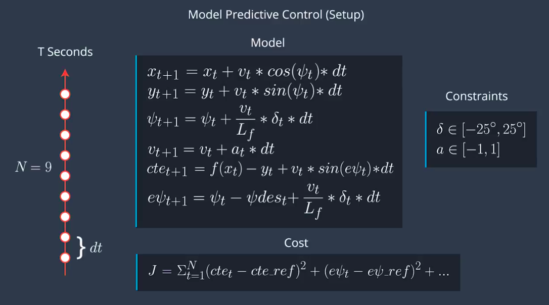
\[ \begin{aligned} x_{t+1}&=x_t+v_t\cos(\psi_t)*dt \\[2mm] y_{t+1}&=y_t+v_t\sin(\psi_t)*dt \\[2mm] \psi_{t+1}&=\psi_t+\frac{v_t}{L_f}\delta*dt \\[2mm] v_{t+1}&=v_t+a_t*dt \end{aligned} \]

\(\begin{bmatrix} x, y, \psi, v \end{bmatrix}\) is the state of the vehicle, \(L_f\) is a physical characteristic of the vehicle, and \(\begin{bmatrix} \delta, a \end{bmatrix}\) are the actuators, or control inputs, to our system.

we add a multiplicative factor of the steering angle, \(\delta\) to \(\psi\). \(L_f\) measures the distance between the center of mass of the vehicle and it's front axle. The larger the vehicle, the slower the turn rate.
If you've driven a vehicle you're well aware at higher speeds you turn quicker than at lower speeds. This is why \(v\) is the included in the update.

Errors

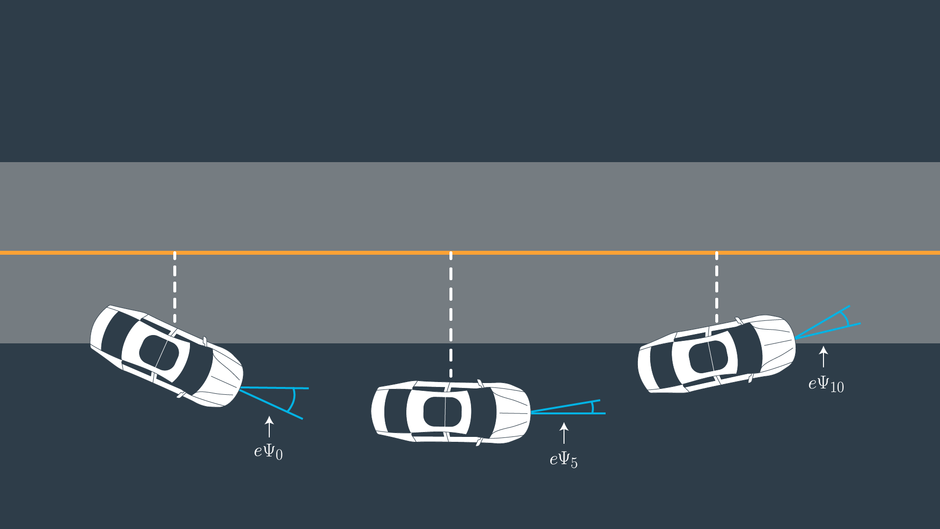
We can capture how the errors we are interested in change over time by deriving our kinematic model around these errors as our new state vector. The new state is \( \begin{pmatrix} x, y, \psi, v, cte, e\psi \end{pmatrix}\).

\[ \begin{aligned} cte_{t+1}&=f(x_t)-y_t+(v_t*\sin(e\psi_t)*dt) \\[2mm] e\psi_{t+1}&=\psi_t-\psi des_t + (\frac{v_t}{L_f}*\delta t*dt) \end{aligned} \]

double cost = 0;
for (int t = 0; t < N; ++t) {
  cost += pow(cte[t], 2);
  cost += pow(epsi[t], 2);
}

还可以添加很多其他误差项。例如方向盘、油门刹车的变化不能太剧烈：

for (int t = 0; t < N-1; ++t) {
  cost += pow(delta[t], 2);
}

for (int t = 0; t < N-1; ++t) {
  cost += pow(delta[t+1] - delta[t], 2);
  cost += pow(a[t+1] - a[t], 2);
}

Dynamic Model

Dynamic Model 精度更高，但是需要考虑各种力学模型，建模也比Kinematic Model 更为复杂。 A dynamic model considers: tire forces, longitudinal and lateral forces, gravity, air resistance, drag.

What we have learned so far From the previous lessons we have learned to apply the bicycle model, polynomial fitting, low complexity heuristics (e.g. CTE), and short time steps, to enable vehicles to follow a complex (polynomial) trajectories. This is an effective, practical, and commonly used approach, which can be applied to many autonomous vehicle scenarios, in real time.

Coming Next For the next few lessons we will round out our discussion of vehicle models with an overview of the more comprehensive, but less practical, dynamic models. Dynamic models and the elements which comprise them are rigorous and could be modules or courses unto themselves. The content that follows is targeted developing awareness and intuition that can be applied to further study and consists of:

• Dynamic Model Forces
• Tire Slip Angle
• Tire Slip Ratio
• Tire Models

Additional resources are linked to each lesson to encourage and enable more in depth study. One of these resources makes a good case for the use of lower complexity kinematic models, as:

Compared to higher fidelity vehicle models, the system identification on the kinematic bicycle model is easier because there are only two parameters to identify, lf and lr. This makes it simpler to port the same controller or path planner to other vehicles with differently sized wheelbases.

To further expand on this, lower complexity models have two strong advantages over higher complexity (dynamic included) models. They can run in real time (essential requirement of any model operating in a vehicle) and they are transferable to vehicles with differing attributes, such as mass. To use a dynamic model engineers would have to be able to control the vehicle attributes of the vehicles they are deploying models into (they probably won't have control over this). High complexity models would need major re-adjustment to account for even small differences. Lower complexity models do not suffer from this constraint and so can be placed in a wider range of vehicles, with far less additional effort, and unpredictability.

Another frequently asked question is where our model comes from and why it differs from other models seen in the program and from other sources.

The kinematic model we derive and use here is not quite the same as in the Berkeley paper (linked above), although they are similar. It is possible to use different models in different parts of your pipeline, depending on what levels of accuracy you need in different places. It is common to see this in industry. The principles of model we present can be applied to add parameters into the model to make models fit to purpose.

Additional Reading

• Pacejka Tire Model
• This paper presents a comparison between a kinematic and dynamic model.
• A brief overview of essential topics in vehicle dynamics
• Drew Gray's dissertation thesis This contains an excellent review, additional resources, and novel approaches/findings.
• An excellent book This is not a free resource but is highly recommended by domain experts.

MPC原理

约束条件

约束条件即为运动学方程，转换成等式，上下界都为0。对应的代码：

size_t n_constraints = 6 * N;

Dvector constraints_lowerbound(n_constraints);
Dvector constraints_upperbound(n_constraints);
for (i = 0; i < n_constraints; i++) {
  constraints_lowerbound[i] = 0;
  constraints_upperbound[i] = 0;
}

constraints_lowerbound[x_start] = constraints_upperbound[x_start] = state[0];
constraints_lowerbound[y_start] = constraints_upperbound[y_start] = state[1];
constraints_lowerbound[psi_start] = constraints_upperbound[psi_start] = state[2];
constraints_lowerbound[v_start] = constraints_upperbound[v_start] = state[3];
constraints_lowerbound[cte_start] = constraints_upperbound[cte_start] = state[4];
constraints_lowerbound[epsi_start] = constraints_upperbound[epsi_start] = state[5];

待估变量

变量包括： \([x,y,\psi,v,cte,e\psi]\)，外加N个时刻的\([\delta, a]\)。对应的代码：

size_t n_vars = 6 * N + 2 * (N - 1);

Dvector vars(n_vars);
for (i = 0; i < n_vars; i++) {
  vars[i] = 0;
}

for (i = delta_start; i < a_start; i++) {
  vars_lowerbound[i] = -0.436332;
  vars_upperbound[i] = 0.436332;
}

for (i = a_start; i < n_vars; i++) {
  vars_lowerbound[i] = -1.0;
  vars_upperbound[i] = 1.0;
}

残差

残差为：

// The part of the cost based on the reference state.
for (size_t t = 0; t < N; t++) {
  fg[0] += 1000 * CppAD::pow(vars[cte_start + t], 2);
  fg[0] += 1000 * CppAD::pow(vars[epsi_start + t], 2);
  fg[0] += CppAD::pow(vars[v_start + t] - ref_v, 2);
}

// Minimize the use of actuators.
for (size_t t = 0; t < N - 1; t++) {
  fg[0] += CppAD::pow(vars[delta_start + t], 2);
  fg[0] += CppAD::pow(vars[a_start + t], 2);
}

// Minimize the value gap between sequential actuations.
for (size_t t = 0; t < N - 2; t++) {
  fg[0] += 500 * CppAD::pow(vars[delta_start + t + 1] - vars[delta_start + t], 2);
  fg[0] += 500 * CppAD::pow(vars[a_start + t + 1] - vars[a_start + t], 2);
}

动力学方程

运动学方程，构建了各个变量之间的数学关系。

// Initialize the model to the initial state
fg[1 + x_start] = vars[x_start];
fg[1 + y_start] = vars[y_start];
fg[1 + psi_start] = vars[psi_start];
fg[1 + v_start] = vars[v_start];
fg[1 + cte_start] = vars[cte_start];
fg[1 + epsi_start] = vars[epsi_start];

for (size_t t = 1; t < N; t++) {
  // The state at time t+1 .
  AD<double> x1 = vars[x_start + t];
  AD<double> y1 = vars[y_start + t];
  AD<double> psi1 = vars[psi_start + t];
  AD<double> v1 = vars[v_start + t];
  AD<double> cte1 = vars[cte_start + t];
  AD<double> epsi1 = vars[epsi_start + t];

  // The state at time t.
  AD<double> x0 = vars[x_start + t - 1];
  AD<double> y0 = vars[y_start + t - 1];
  AD<double> psi0 = vars[psi_start + t - 1];
  AD<double> v0 = vars[v_start + t - 1];
  AD<double> cte0 = vars[cte_start + t - 1];
  AD<double> epsi0 = vars[epsi_start + t - 1];

  // Only consider the actuation at time t.
  AD<double> delta0 = vars[delta_start + t - 1];
  AD<double> a0 = vars[a_start + t - 1];

  AD<double> f0 = coeffs[0] + coeffs[1]*x0 + coeffs[2]*x0*x0 + coeffs[3]*x0*x0*x0;
  AD<double> psides0 = CppAD::atan(3*coeffs[3]*x0*x0 + 2*coeffs[2]*x0 + coeffs[1]);
  /* AD<double> f0 = coeffs[0] + coeffs[1] * x0; */
  /* AD<double> psides0 = CppAD::atan(coeffs[1]); */

  // Here's `x` to get you started.
  // The idea here is to constraint this value to be 0.
  fg[1 + x_start + t] = x1 - (x0 + v0 * CppAD::cos(psi0) * dt);
  fg[1 + y_start + t] = y1 - (y0 + v0 * CppAD::sin(psi0) * dt);
  fg[1 + psi_start + t] = psi1 - (psi0 - v0 * delta0 / Lf * dt);
  fg[1 + v_start + t] = v1 - (v0 + a0 * dt);
  fg[1 + cte_start + t] = cte1 - ((f0 - y0) + (v0 * CppAD::sin(epsi0) * dt));
  fg[1 + epsi_start + t] = epsi1 - ((psi0 - psides0) - v0 * delta0 / Lf * dt);
}

优化器

Ipopt (Interior Point OPTimizer, pronounced eye-pea-Opt) is a software package for large-scale nonlinear optimization. It is designed to find (local) solutions of mathematical optimization problems. Ipopt is the tool we'll be using to optimize the control inputs.

CppAD (C++ Algorithmic Differentiation Package) is a library we'll use for automatic differentiation. By using CppAD we don't have to manually compute derivatives, which is tedious and prone to error.